Last year I wrote about eight databases that support in-database machine learning. In-database machine learning is important because it brings the machine learning processing to the data, which is much more efficient for big data, rather than forcing data scientists to extract subsets of the data to where the machine learning training and inference run.
These databases each work in a different way:
- Amazon Redshift ML uses SageMaker Autopilot to automatically create prediction models from the data you specify via a SQL statement, which is extracted to an Amazon S3 bucket. The best prediction function found is registered in the Redshift cluster.
- BlazingSQL can run GPU-accelerated queries on data lakes in Amazon S3, pass the resulting DataFrames to RAPIDS cuDF for data manipulation, and finally perform machine learning with RAPIDS XGBoost and cuML, and deep learning with PyTorch and TensorFlow.
- BigQuery ML brings much of the power of Google Cloud Machine Learning into the BigQuery data warehouse with SQL syntax, without extracting the data from the data warehouse.
- IBM Db2 Warehouse includes a wide set of in-database SQL analytics that includes some basic machine learning functionality, plus in-database support for R and Python.
- Kinetica provides a full in-database lifecycle solution for machine learning accelerated by GPUs, and can calculate features from streaming data.
- Microsoft SQL Server can train and infer machine learning models in multiple programming languages.
- Oracle Cloud Infrastructure can host data science resources integrated with its data warehouse, object store, and functions, allowing for a full model development lifecycle.
- Vertica has a nice set of machine learning algorithms built-in, and can import TensorFlow and PMML models. It can do prediction from imported models as well as its own models.
Now there’s another database that can run machine learning internally: Snowflake.
Snowflake overview
Snowflake is a fully relational ANSI SQL enterprise data warehouse that was built from the ground up for the cloud. Its architecture separates compute from storage so that you can scale up and down on the fly, without delay or disruption, even while queries are running. You get the performance you need exactly when you need it, and you only pay for the compute you use.
Snowflake currently runs on Amazon Web Services, Microsoft Azure, and Google Cloud Platform. It has recently added External Tables On-Premises Storage, which lets Snowflake users access their data in on-premises storage systems from companies including Dell Technologies and Pure Storage, expanding Snowflake beyond its cloud-only roots.
Snowflake is a fully columnar database with vectorized execution, making it capable of addressing even the most demanding analytic workloads. Snowflake’s adaptive optimization ensures that queries automatically get the best performance possible, with no indexes, distribution keys, or tuning parameters to manage.
Snowflake can support unlimited concurrency with its unique multi-cluster, shared data architecture. This allows multiple compute clusters to operate simultaneously on the same data without degrading performance. Snowflake can even scale automatically to handle varying concurrency demands with its multi-cluster virtual warehouse feature, transparently adding compute resources during peak load periods and scaling down when loads subside.
Snowpark overview
When I reviewed Snowflake in 2019, if you wanted to program against its API you needed to run the program outside of Snowflake and connect through ODBC or JDBC drivers or through native connectors for programming languages. That changed with the introduction of Snowpark in 2021.
Snowpark brings to Snowflake deeply integrated, DataFrame-style programming in the languages developers like to use, starting with Scala, then extending to Java and now Python. Snowpark is designed to make building complex data pipelines a breeze and to allow developers to interact with Snowflake directly without moving data.
The Snowpark library provides an intuitive API for querying and processing data in a data pipeline. Using this library, you can build applications that process data in Snowflake without moving data to the system where your application code runs.
The Snowpark API provides programming language constructs for building SQL statements. For example, the API provides a select method that you can use to specify the column names to return, rather than writing ‘select column_name’ as a string. Although you can still use a string to specify the SQL statement to execute, you benefit from features like intelligent code completion and type checking when you use the native language constructs provided by Snowpark.
Snowpark operations are executed lazily on the server, which reduces the amount of data transferred between your client and the Snowflake database. The core abstraction in Snowpark is the DataFrame, which represents a set of data and provides methods to operate on that data. In your client code, you construct a DataFrame object and set it up to retrieve the data that you want to use.
The data isn’t retrieved at the time when you construct the DataFrame object. Instead, when you are ready to retrieve the data, you can perform an action that evaluates the DataFrame objects and sends the corresponding SQL statements to the Snowflake database for execution.
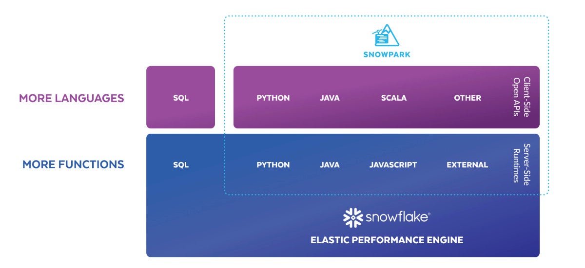
Snowpark block diagram. Snowpark expands the internal programmability of the Snowflake cloud data warehouse from SQL to Python, Java, Scala, and other programming languages.
Snowpark for Python overview
Snowpark for Python is available in public preview to all Snowflake customers, as of June 14, 2022. In addition to the Snowpark Python API and Python Scalar User Defined Functions (UDFs), Snowpark for Python supports the Python UDF Batch API (Vectorized UDFs), Table Functions (UDTFs), and Stored Procedures.
These features combined with Anaconda integration provide the Python community of data scientists, data engineers, and developers with a variety of flexible programming contracts and access to open source Python packages to build data pipelines and machine learning workflows directly within Snowflake.
Snowpark for Python includes a local development experience you can install on your own machine, including a Snowflake channel on the Conda repository. You can use your preferred Python IDEs and dev tools and be able to upload your code to Snowflake knowing that it will be compatible.
By the way, Snowpark for Python is free open source. That’s a change from Snowflake’s history of keeping its code proprietary.
The following sample Snowpark for Python code creates a DataFrame that aggregates book sales by year. Under the hood, DataFrame operations are transparently converted into SQL queries that get pushed down to the Snowflake SQL engine.
from snowflake.snowpark import Session
from snowflake.snowpark.functions import col
# fetch snowflake connection information
from config import connection_parameters
# build connection to Snowflake
session = Session.builder.configs(connection_parameters).create()
# use Snowpark API to aggregate book sales by year
booksales_df = session.table(“sales”)
booksales_by_year_df = booksales_df.groupBy(year(“sold_time_stamp”)).agg([(col(“qty”),”count”)]).sort(“count”, ascending=False)
booksales_by_year_df.show()
Getting started with Snowpark Python
Snowflake’s “getting started” tutorial demonstrates an end-to-end data science workflow using Snowpark for Python to load, clean, and prepare data and then deploy the trained model to Snowflake using a Python UDF for inference. In 45 minutes (nominally), it teaches:
- How to create a DataFrame that loads data from a stage;
- How to perform data and feature engineering using the Snowpark DataFrame API; and
- How to bring a trained machine learning model into Snowflake as a UDF to score new data.
The task is the classic customer churn prediction for an internet service provider, which is a straightforward binary classification problem. The tutorial starts with a local setup phase using Anaconda; I installed Miniconda for that. It took longer than I expected to download and install all the dependencies of the Snowpark API, but that worked fine, and I appreciate the way Conda environments avoid clashes among libraries and versions.
This quickstart begins with a single Parquet file of raw data and extracts, transforms, and loads the relevant information into multiple Snowflake tables.
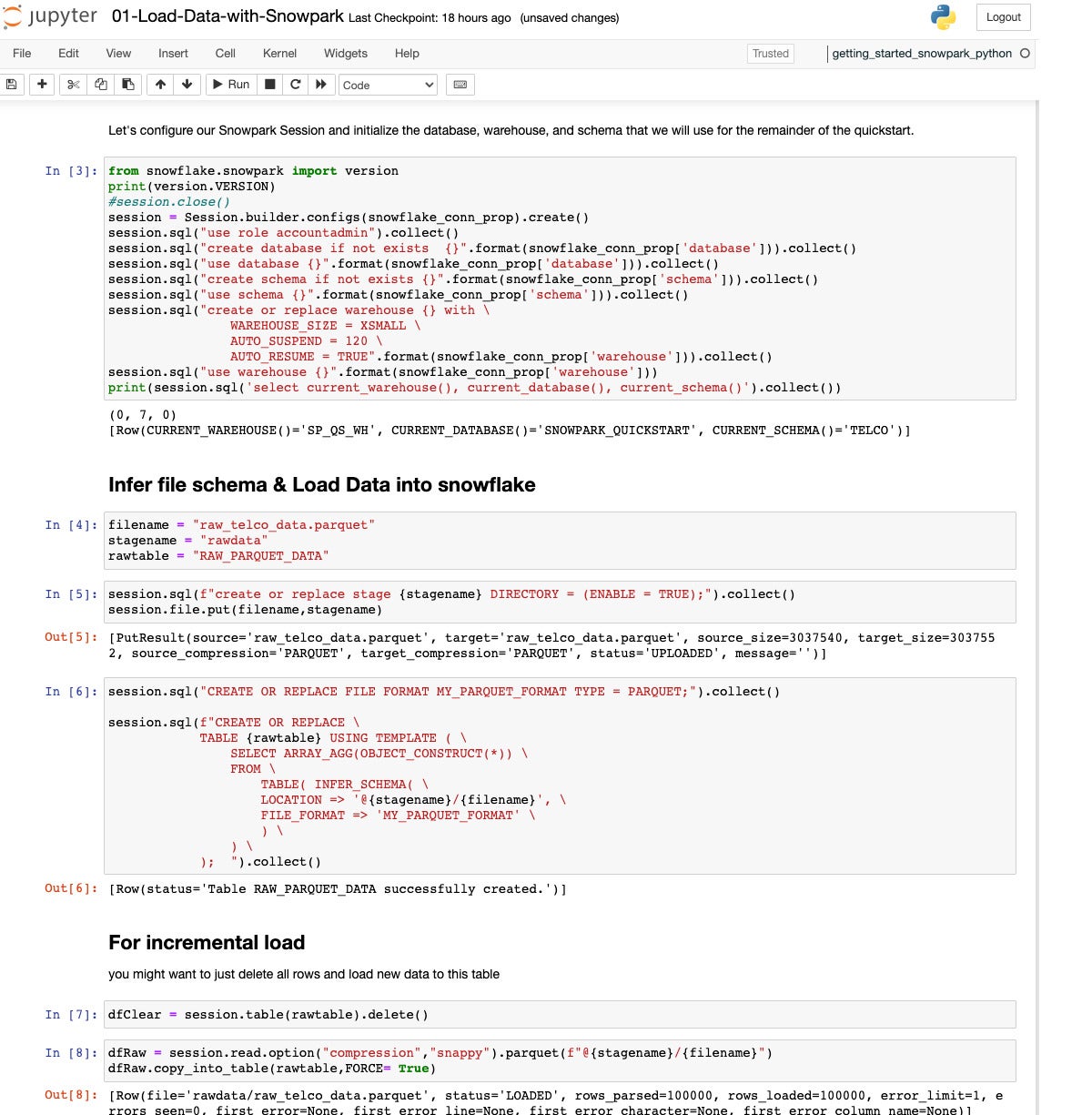
We’re looking at the beginning of the “Load Data with Snowpark” quickstart. This is a Python Jupyter Notebook running on my MacBook Pro that calls out to Snowflake and uses the Snowpark API. Step 3 originally gave me problems, because I wasn’t clear from the documentation about where to find my account ID and how much of it to include in the account field of the config file. For future reference, look in the “Welcome To Snowflake!” email for your account information.
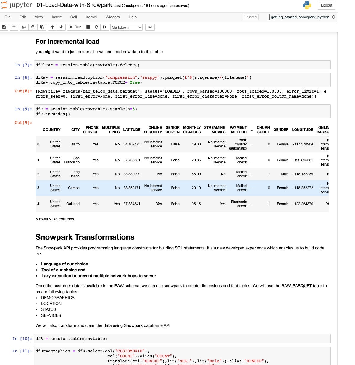
Here we are checking the loaded table of raw historical customer data and beginning to set up some transformations.
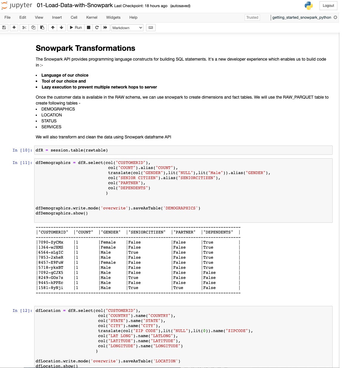
Here we’ve extracted and transformed the demographics data into its own DataFrame and saved that as a table.
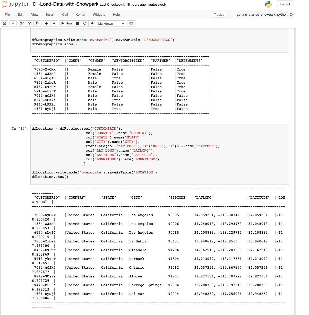
In step 12, we extract and transform the fields for a location table. As before, this is done with a SQL query into a DataFrame, which is then saved as a table.
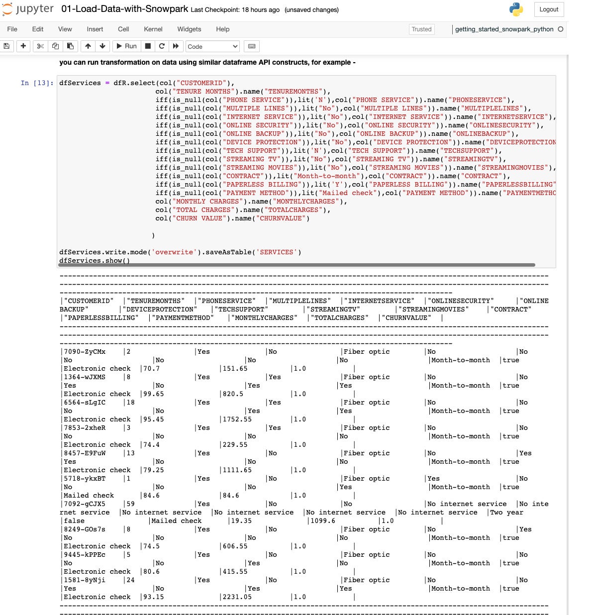
Here we extract and transform data from the raw DataFrame into a Services table in Snowflake.
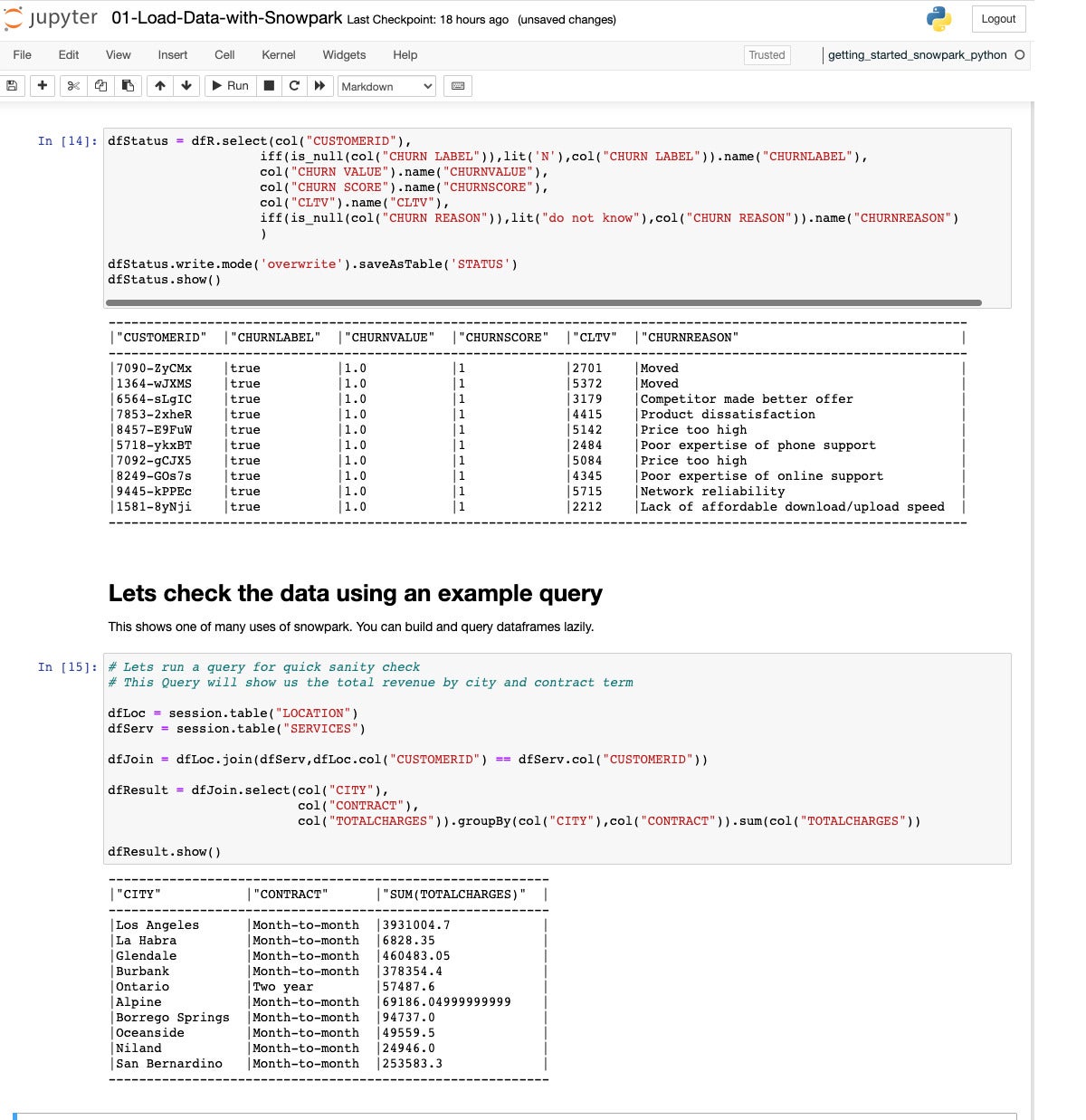
Next we extract, transform, and load the final table, Status, which shows the churn status and the reason for leaving. Then we do a quick sanity check, joining the Location and Services tables into a Join DataFrame, then aggregating total charges by city and type of contract for a Result DataFrame.
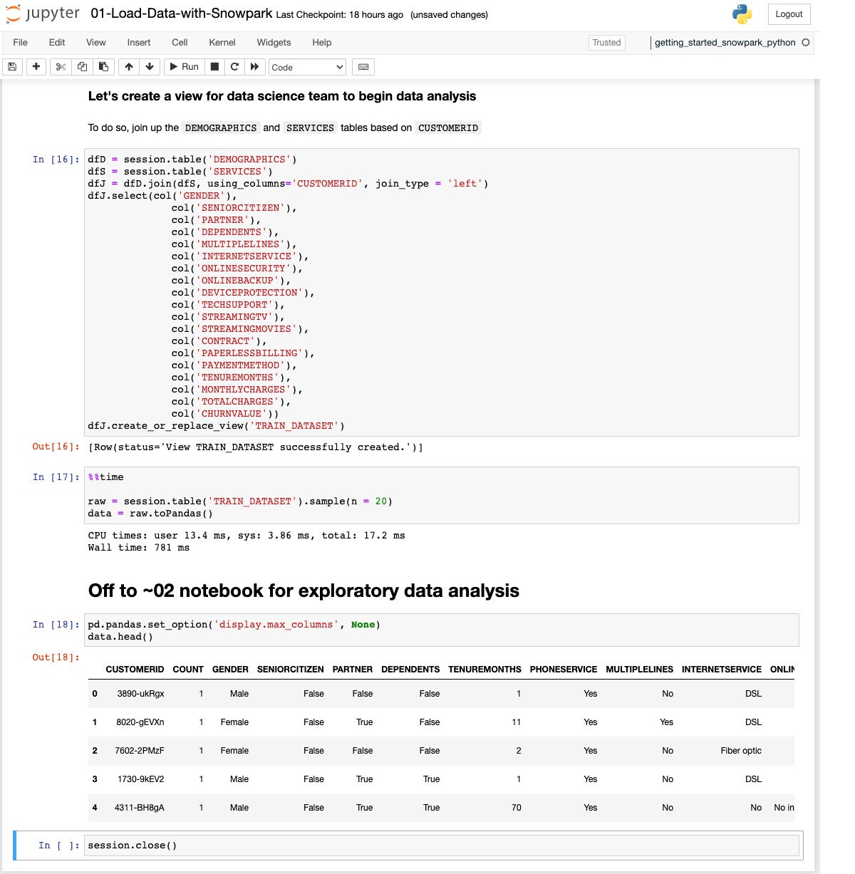
In this step we join the Demographics and Services tables to create a TRAIN_DATASET view. We use DataFrames for intermediate steps, and use a select statement on the joined DataFrame to reorder the columns.
Now that we’ve finished the ETL/data engineering phase, we can move on to the data analysis/data science phase.
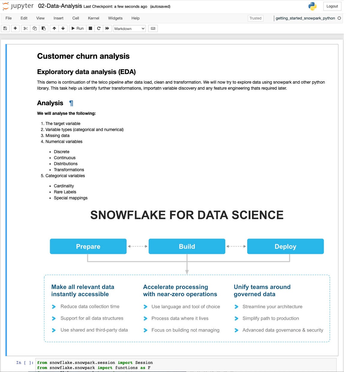
This page introduces the analysis we’re about to perform.
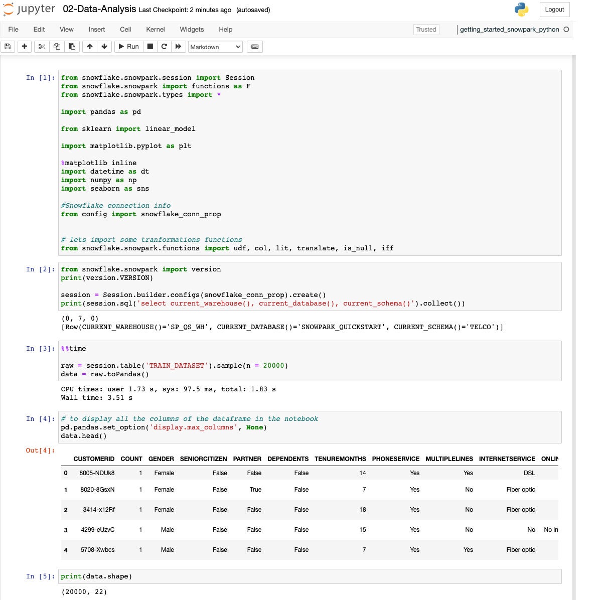
We start by pulling in the Snowpark, Pandas, Scikit-learn, Matplotlib, datetime, NumPy, and Seaborn libraries, as well as reading our configuration. Then we establish our Snowflake database session, sample 10K rows from the TRAIN_DATASET view, and convert that to Pandas format.
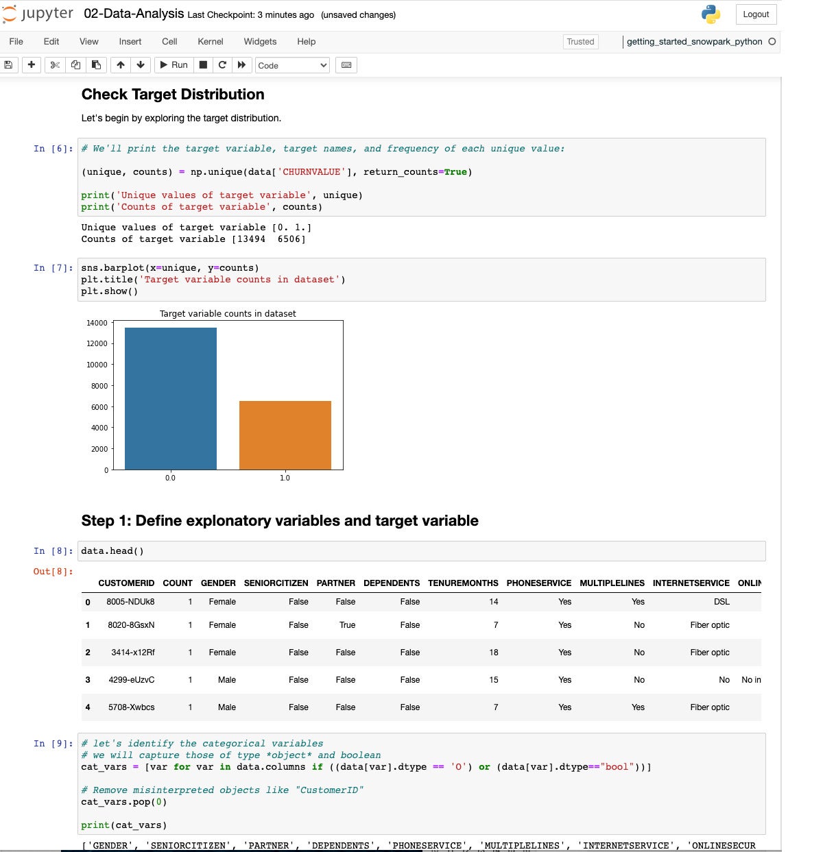
We continue with some exploratory data analysis using NumPy, Seaborn, and Pandas. We look for non-numerical variables and classify them as categories.
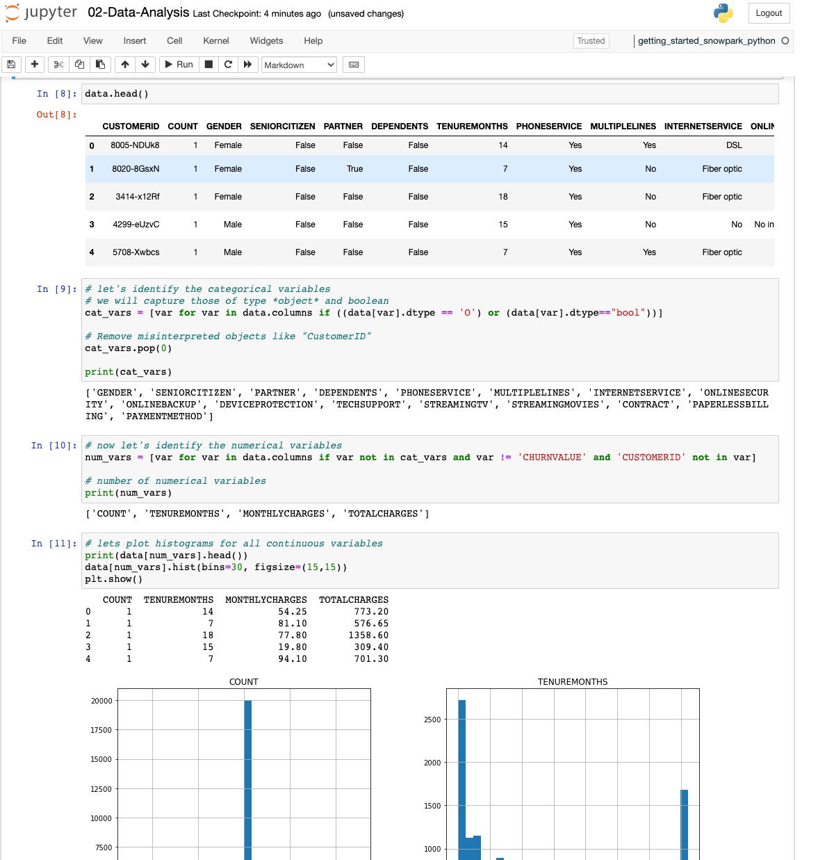
Once we have found the categorical variables, then we identify the numerical variables and plot some histograms to see the distribution.
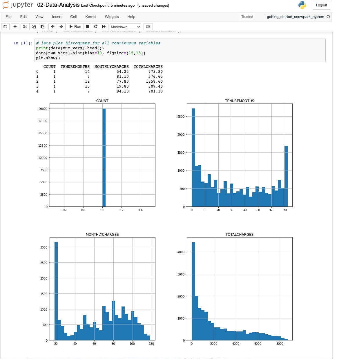
All four histograms.
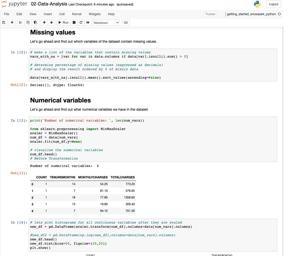
Given the assortment of ranges we saw in the previous screen, we need to scale the variables for use in a model.
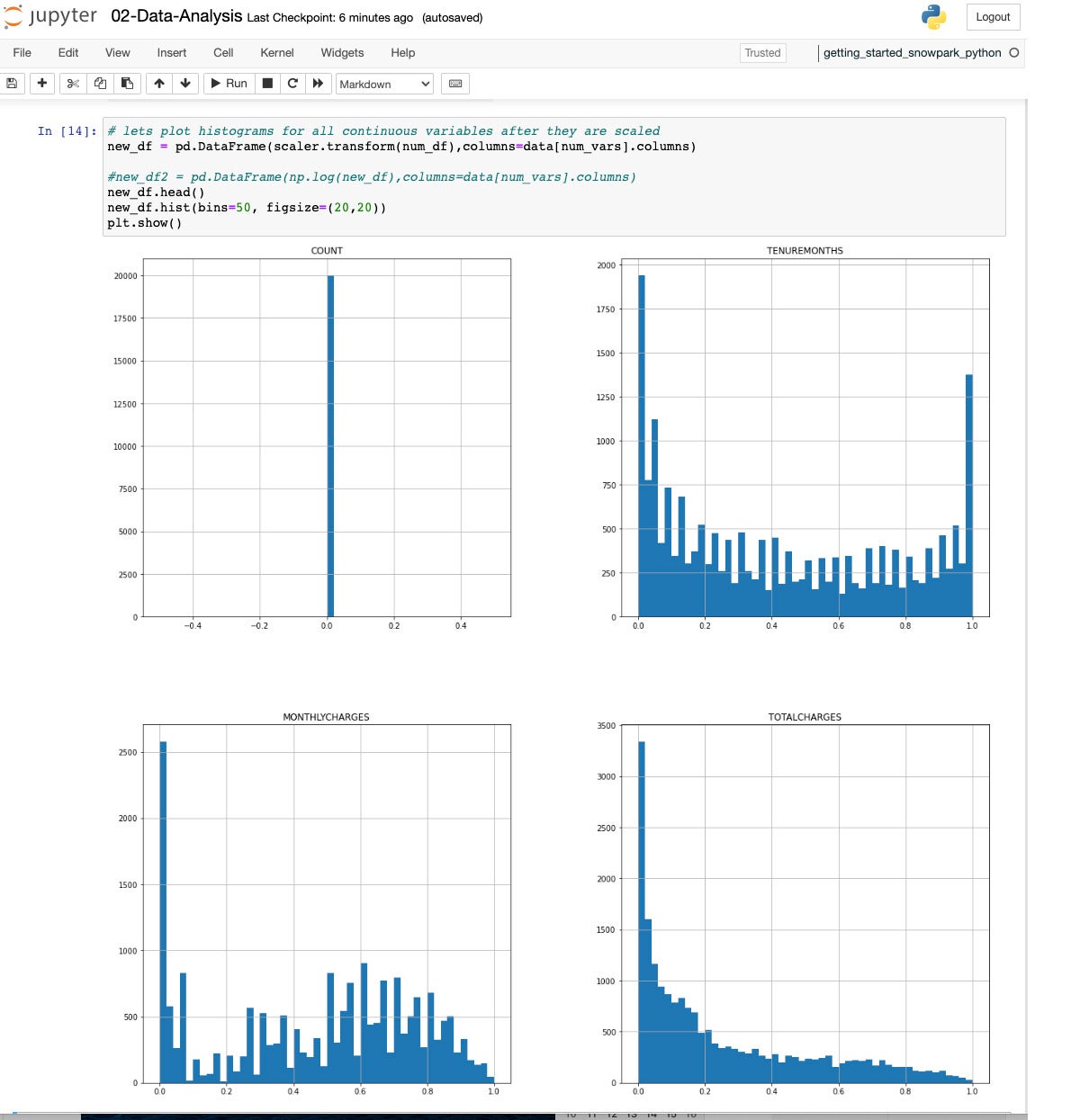
Having all the numerical variables lie in the range from 0 to 1 will help immensely when we build a model.
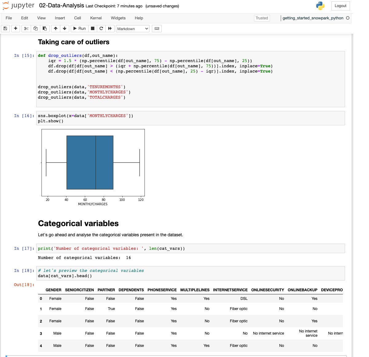
Three of the numerical variables have outliers. Let’s drop them to avoid having them skew the model.
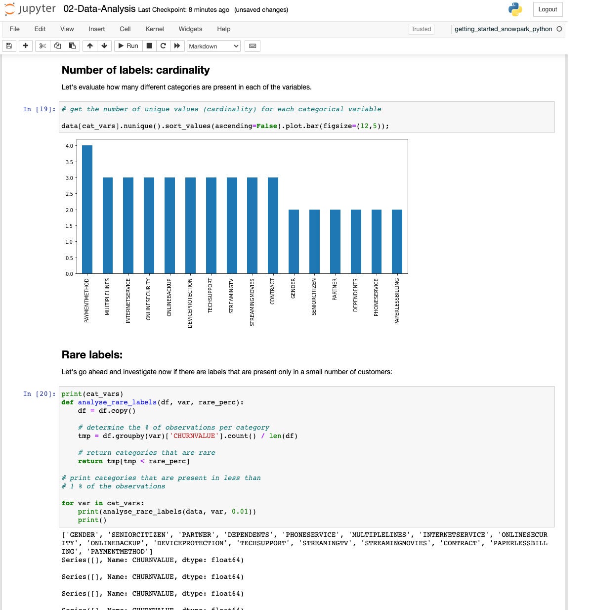
If we look at the cardinality of the categorical variables, we see they range from 2 to 4 categories.
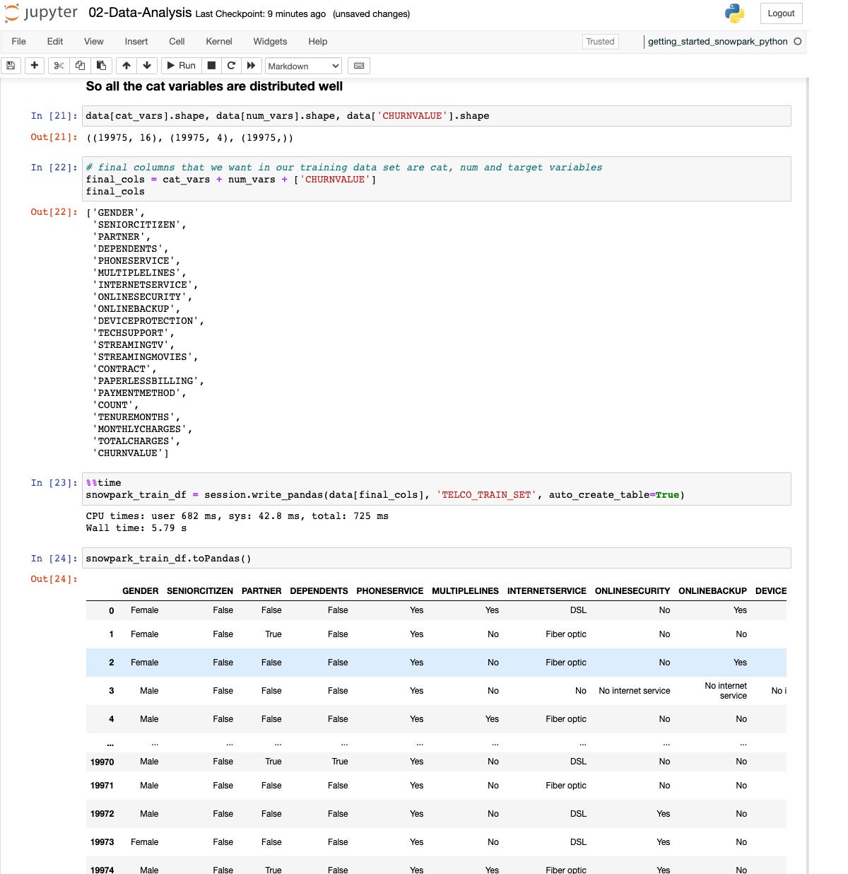
We pick our variables and write the Pandas data out to a Snowflake table, TELCO_TRAIN_SET.
Finally we create and deploy a user-defined function (UDF) for prediction, using more data and a better model.
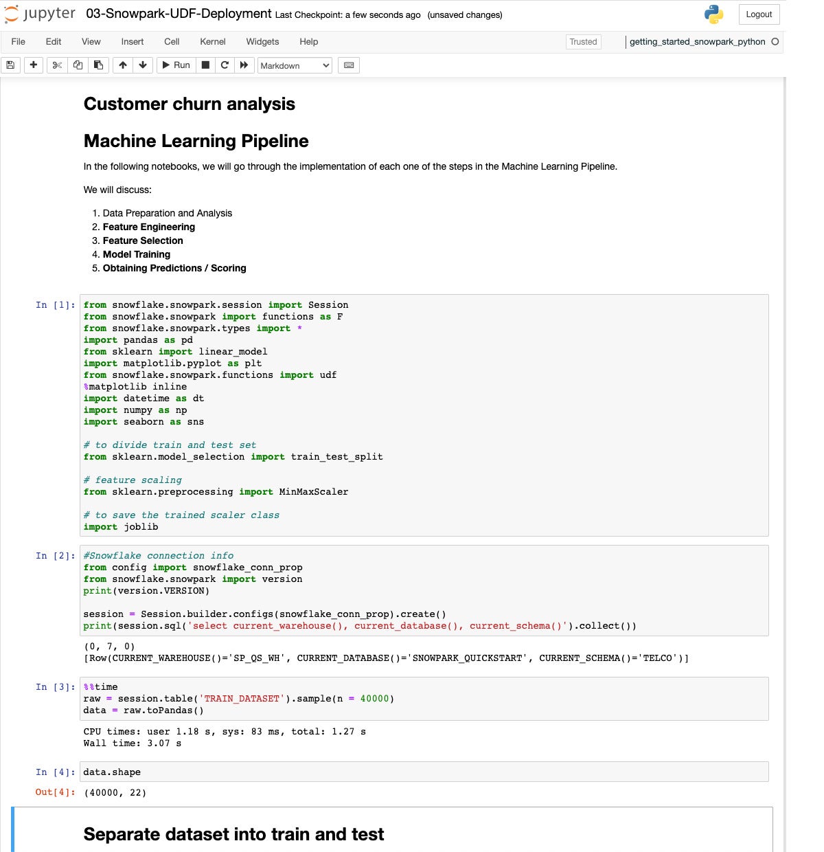
Now we set up for deploying a predictor. This time we sample 40K values from the training dataset.
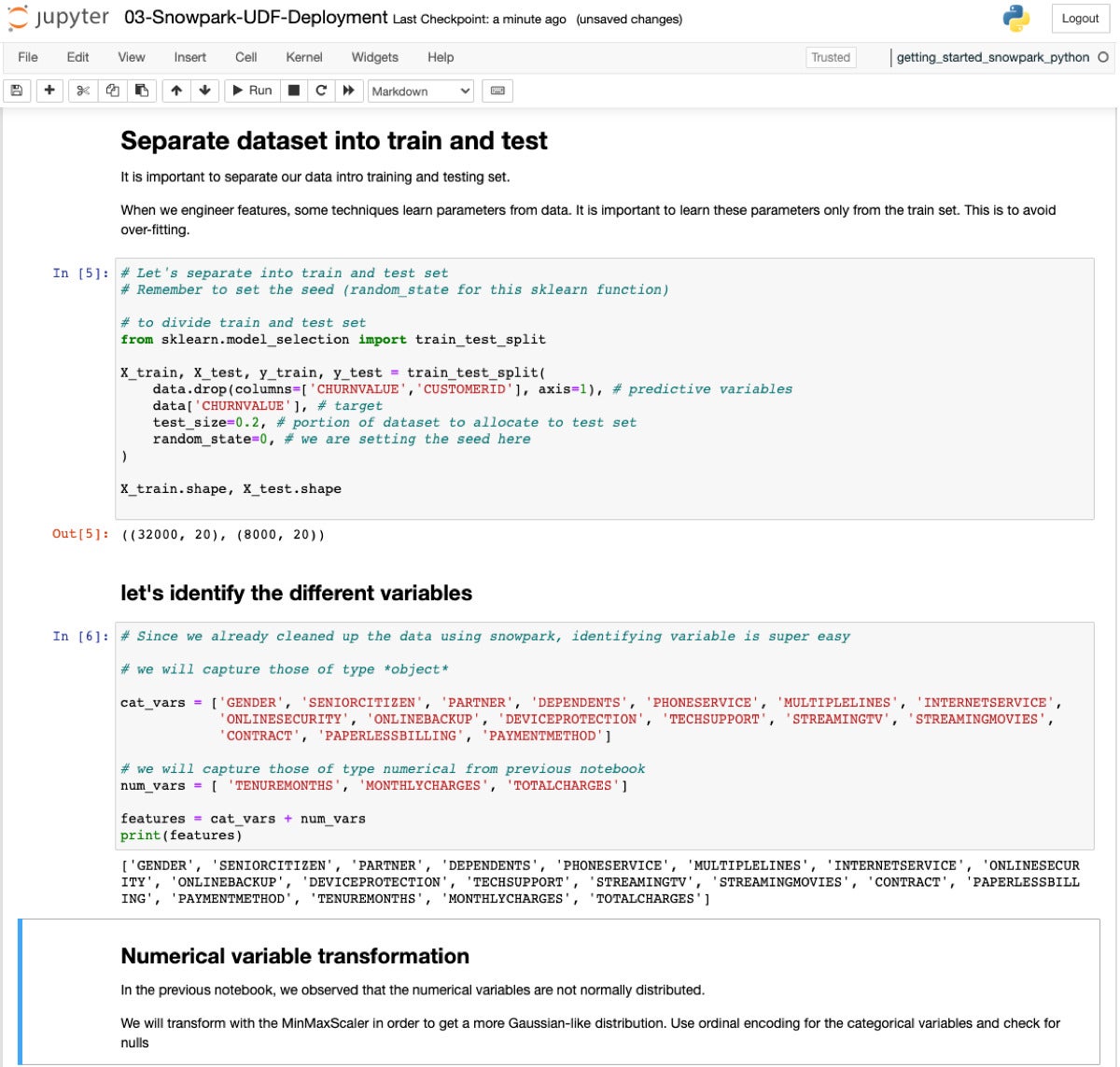
Now we’re setting up for model fitting, on our way to deploying a predictor. Splitting the dataset 80/20 is standard stuff.
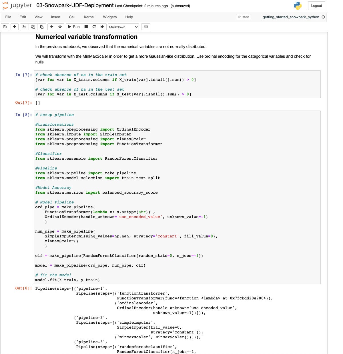
This time we’ll use a Random Forest classifier and set up a Scikit-learn pipeline that handles the data engineering as well as doing the fitting.
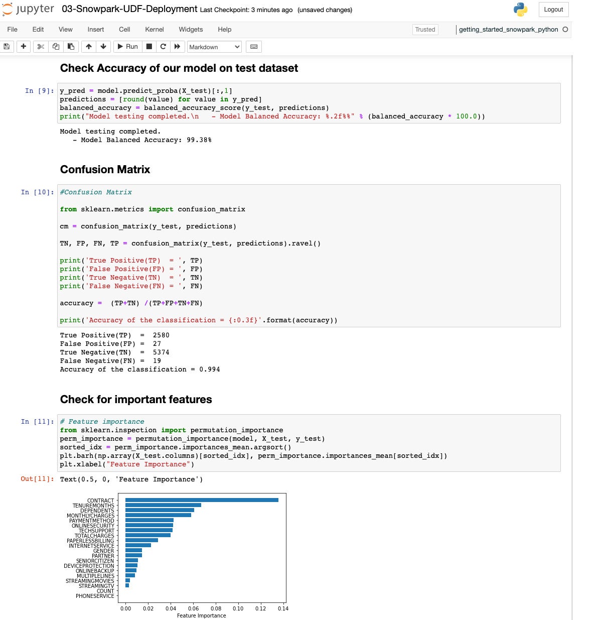
Let’s see how we did. The accuracy is 99.38%, which isn’t shabby, and the confusion matrix shows relatively few false predictions. The most important feature is whether there is a contract, followed by tenure length and monthly charges.
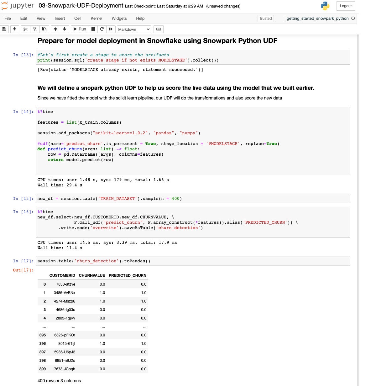
Now we define a UDF to predict churn and deploy it into the data warehouse.
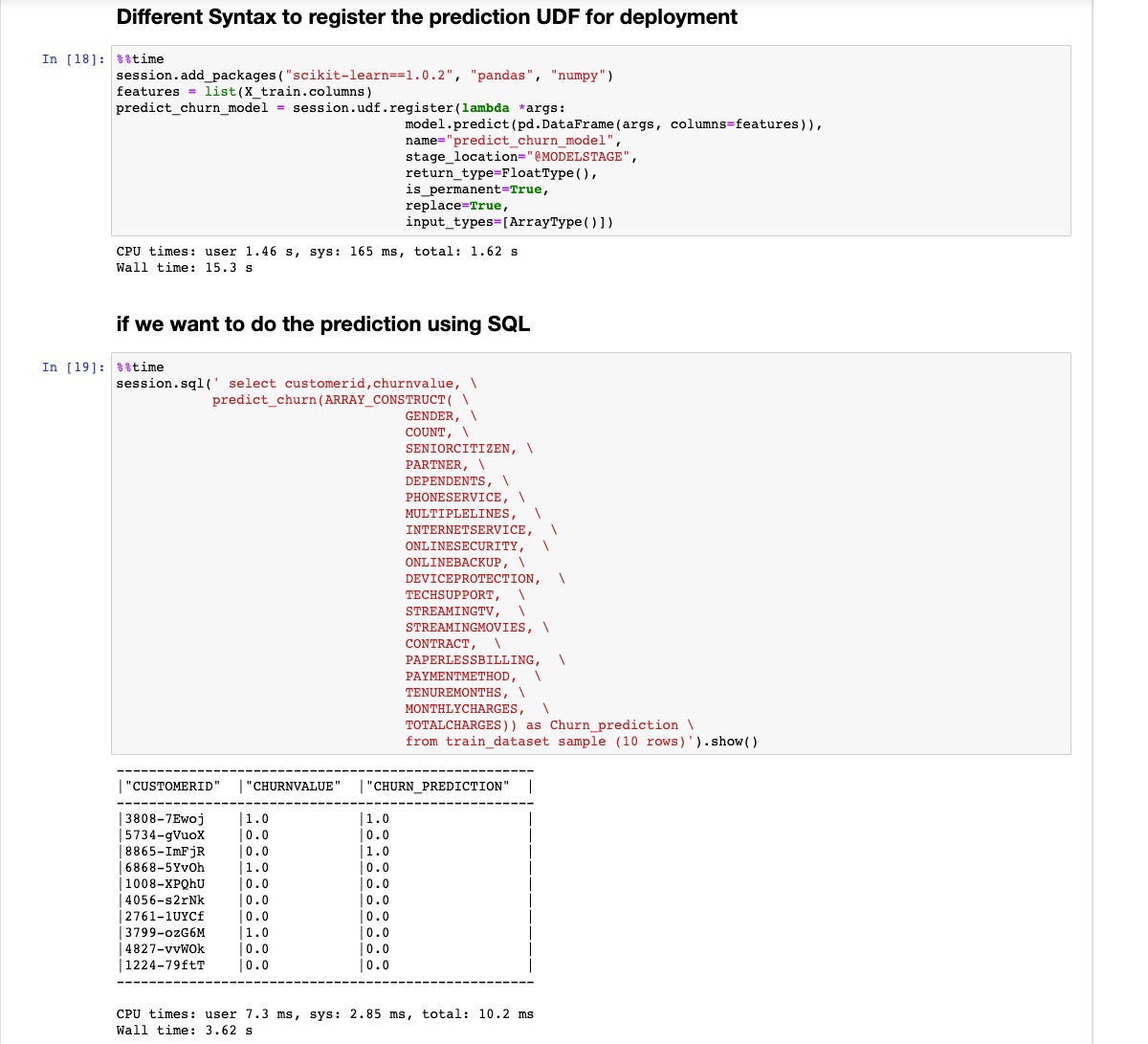
Step 18 shows another way to register the UDF, using session.udf.register() instead of a select statement. Step 19 shows another way to run the prediction function, incorporating it into a SQL select statement instead of a DataFrame select statement.
You can go into more depth by running Machine Learning with Snowpark Python, a 300-level quickstart, which analyzes Citibike rental data and builds an orchestrated end-to-end machine learning pipeline to perform monthly forecasts using Snowflake, Snowpark Python, PyTorch, and Apache Airflow. It also displays results using Streamlit.
Overall, Snowpark for Python is very good. While I stumbled over a couple of things in the quickstart, they were resolved fairly quickly with help from Snowflake’s extensibility support.
I like the wide range of popular Python machine learning and deep learning libraries and frameworks included in the Snowpark for Python installation. I like the way Python code running on my local machine can control Snowflake warehouses dynamically, scaling them up and down at will to control costs and keep runtimes reasonably short. I like the efficiency of doing most of the heavy lifting inside the Snowflake warehouses using Snowpark. I like being able to deploy predictors as UDFs in Snowflake without incurring the costs of deploying prediction endpoints on major cloud services.
Essentially, Snowpark for Python gives data engineers and data scientists a nice way to do DataFrame-style programming against the Snowflake enterprise data warehouse, including the ability to set up full-blown machine learning pipelines to run on a recurrent schedule.
—
Cost: $2 per credit plus $23 per TB per month storage, standard plan, prepaid storage. 1 credit = 1 node*hour, billed by the second. Higher level plans and on-demand storage are more expensive. Data transfer charges are additional, and vary by cloud and region. When a virtual warehouse is not running (i.e., when it is set to sleep mode), it does not consume any Snowflake credits. Serverless features use Snowflake-managed compute resources and consume Snowflake credits when they are used.
Platform: Amazon Web Services, Microsoft Azure, Google Cloud Platform.
Copyright © 2022 IDG Communications, Inc.
Source by www.infoworld.com


